Quickstart

The following is a simple example of using pocoMC to get started. We will sample the infamous Rosenbrock distribution in 10D.

Likelihood function and prior distribution

The first step in any analysis is to define the prior distribution and likelihood function. More precisely, for computational reasons, we require the logarithm of the prior probability density function \(\log\pi(\theta)\equiv \log p(\theta)\) and the logarithm of the likelihood function \(\log \mathcal{L}(\theta)\equiv\log P(d\vert \theta)\).

import numpy as np
from scipy.stats import uniform, norm

# import pocoMC
import pocomc as pc

# Set the random seed.
np.random.seed(0)

# Define the dimensionality of our problem.
n_dim = 10

# Define our 10-D Rosenbrock log-likelihood.
def log_likelihood(x):
    return -np.sum(10.0 * (x[:, ::2] ** 2.0 - x[:, 1::2]) ** 2.0 + (x[:, ::2] - 1.0) ** 2.0, axis=1)

# Define our normal/Gaussian prior.
prior = pc.Prior(n_dim*[norm(0.0, 3.0)]) # N(0,3)

Preconditioned Monte Carlo sampling

The next step is to initialise the PMC sampler using pocoMC and configure it for our analysis.

# Initialise sampler
sampler = pc.Sampler(
    prior=prior,
    likelihood=log_likelihood,
    vectorize=True,
    random_state=0
)

Next, we can start sampling.

# Start sampling
sampler.run()

Iter: 44it [02:56,  4.00s/it, calls=97500, beta=1, logZ=-21.3, ESS=4.66e+3, accept=0.635, steps=3, logp=-14.4, efficiency=1]        

Results

Posterior samples

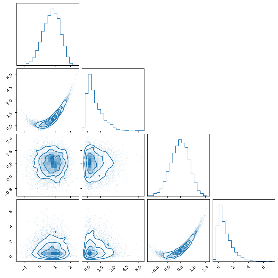
We can get the weighted posterior samples (along with their log-likelihood and log-prior values) using the posterior() method and then plot their 1D and 2D marginal distributions using corner.

import matplotlib.pyplot as plt
import corner

# Get the results
samples, weights, logl, logp = sampler.posterior()

# Trace plot for the first 4 parameters
fig = corner.corner(samples[:,:4], weights=weights, color="C0")
plt.show()

Bayesian Model Evidence or Marginal Likelihood

We can compute the model evidence and its associated uncertainty using the evidence() method.

# Get the evidence and its uncertainty
logz, logz_err = sampler.evidence()

print("logZ", logz, "+-", logz_err)

logZ -21.507899192104063 +- 0.02914336725166582